Using Optimization for Maximizing Future Utility of Ecosystem Services
doi: https://doi.org/10.5552/crojfe.2025.2624
volume: issue, issue:
pp: 20
- Author(s):
-
- Caglayan İnci
- Eriksson Ola
- Ohman Karin
- Yeşil Ahmet
- Bettinger Pete
- Article category:
- Original scientific paper
- Keywords:
- ecosystem services, forest harvest scheduling, optimization, treatment schedules, mixed-integer programming
Abstract
HTML
This study presents a novel, structured optimization approach for incorporating multiple ecosystem services (ES) into long-term strategic and tactical forest management planning. We provide a new and improved framework for forest planning based on ecosystem values of education, aesthetics, cultural heritage, recreation, carbon, water regulation, and water supply. First, the suitability values of seven ecosystem services (ES) were estimated to produce timber harvest and store carbon under fifty potential treatment schedules over a 100-year planning horizon. Then optimization was applied to maximize future utility values derived from values of ES that can be developed with treatment schedules and using the weights of the Sustainable Development Goals (SDG). Finally, the model defined ES functions that were weight-adjusted to select a successful scenario. Thus, we demonstrated that our approach could generate the optimal future suitability value of ES for long-term forest planning compared to the current value of ES. The results showed that the ES that is most affected when harvest demand and harvest flow constraints change is carbon. The value of other ES did not change when scheduled timber volume changed, and as a result we suggest that standing volume and growth increment be considered as criteria used to determine the future value of other ES. We found that the development of suitable value-effective management strategies for securing forest ES values in future stand developments was possible while also achieving other goals and while also being constrained by operational considerations. Our study therefore contributes to ongoing debates about the management of ES.
Using Optimization for Maximizing Future Utility of Ecosystem Services
İnci Caglayan, Ola Eriksson, Karin Ohman, Ahmet Yeşil, Pete Bettinger
https://doi.org/10.5552/crojfe.2025.2624
Abstract
This study presents a novel, structured optimization approach for incorporating multiple ecosystem services (ES) into long-term strategic and tactical forest management planning. We provide a new and improved framework for forest planning based on ecosystem values of education, aesthetics, cultural heritage, recreation, carbon, water regulation, and water supply. First, the suitability values of seven ecosystem services (ES) were estimated to produce timber harvest and store carbon under fifty potential treatment schedules over a 100-year planning horizon. Then optimization was applied to maximize future utility values derived from values of ES that can be developed with treatment schedules and using the weights of the Sustainable Development Goals (SDG). Finally, the model defined ES functions that were weight-adjusted to select a successful scenario. Thus, we demonstrated that our approach could generate the optimal future suitability value of ES for long-term forest planning compared to the current value of ES. The results showed that the ES that is most affected when harvest demand and harvest flow constraints change is carbon. The value of other ES did not change when scheduled timber volume changed, and as a result we suggest that standing volume and growth increment be considered as criteria used to determine the future value of other ES. We found that the development of suitable value-effective management strategies for securing forest ES values in future stand developments was possible while also achieving other goals and while also being constrained by operational considerations. Our study therefore contributes to ongoing debates about the management of ES.
Keywords: ecosystem services, forest harvest scheduling, optimization, treatment schedules, mixed-integer programming
1. Introduction
Ecosystem services (ES) provide goods and services that are essential for human well-being and environmental health (Costanza et al. 1997, MEA 2005). Forests provide multiple ES, which are generally classified as provisioning (e.g., timber, water supply), regulating (e.g., carbon, soil quality, water regulation), supporting (e.g., photosynthesis, soil formation, nutrient cycling), and cultural services (e.g., recreation, aesthetic, cultural heritage value) (Haines-Young and Potschin 2012). However, some forest ecosystems have been constantly degraded because of increasing human demands for firewood, timber, pasture, shelter, recreation, etc. (ITTO 2002, Köchli and Brang 2005, Liu et al. 2007). To prevent further degradation, some forest management plans, policies, and programs have been designed in line with the concept of ES (Wenhua 2004).
Some government agencies, private landowners, and companies have adopted the concept of managing forests for ES (Martinez-Harms et al. 2015, Juerges et al. 2020). As awareness grows about the interdependence of ES and society, pressures grow worldwide for a need for collaborative planning of forest resources (Baskent et al. 2020). The concept of being guided by the development and maintenance of ES in natural resources management can improve the efficient use of resources (Ostrom 2009, Wainger et al. 2010). Despite these societal pressures, forest managers in both the private and public sectors have lagged behind incorporating these benefits into planning. The type of planning process needed brings with it several complexities and challenges (Chan et al. 2006, Haara et al. 2018, Saarikoski et al. 2018). In Türkiye, the Forest Planning Department of the GDF (General Directory of Forestry) has adopted the concept of ES. Therefore, Türkiye’s forests have been managed according to ecosystem based multi-functional management plans since 2008. In the current system, forest ES are determined according to objective criteria and indicators but quantitative decision making techniques are not used in the planning phase. The absence of any planning method based on the concept of ES raises the question of how to plan and manage efficiently ES.
Scientific research on the multi-functional management of forest ES may include stages that define ES, quantify the value of ES, develop strategies for being guided by the development and maintenance of ES, and that integrate these strategies into optimization processes (Başkent 2018). In some cases, decision support tools have been developed for each of those stages. With the rapid growth of research in mapping and assessing ES (Costanza et al. 1997, Egoh et al. 2012, Grêt-Regamey et al. 2015, Maes et al. 2013, Martinez-Harms et al. 2015, Nikodinoska et al. 2018), different assessment methods and tools (Boumans and Costanza 2007, Bagstad et al. 2011, Sharp et al. 2014, Hu et al. 2015) have emerged. Defining effective management practices for environmental management includes recognizing interactions, tradeoffs, or synergies of ES (Bennett et al. 2009, Garcia-Gonzalo et al. 2015, Seidl et al. 2013). Using a Geographical Information System (GIS), many studies have illustrated the tradeoffs between multiple ES between different management scenarios (Cademus et al. 2014, Hu et al. 2015, Bottalico et al. 2016, Vizzarri et al. 2017). This mapping and assessment of ES is also the first step in determining the criteria sets for multi-criteria decision analysis (MCDA) based planning approaches. Geneletti (2011) considers the mapping of ES and the creation of indicators as one of the ways to manage information in integrating ES into spatial planning. However, criteria and indicators may be developed locally for the assessment of ES based on multi-functional management plans (Zengin et al. 2013, Başkent 2018). Furthermore, these assessments inform us about the value of ES and can be used as data in the development of management plans. However, simply using the assessment of forest ES is not sufficient for the strategic planning of the forest ecosystem. Since the forests have a dynamic structure, the value of the ES in forests will change over time after silvicultural treatments are applied (Marchi et al. 2018). The planner needs to observe how these values will change and then suggest the appropriate treatments based on these changes. Classic forest planning approaches, which are typically tactical in nature, focus mainly on timber production and do not incorporate dynamic evaluations of ecosystem services (ES) under different treatment schedules. A strategic planning approach, on the other hand, allows for assessing how ES values evolve over time under alternative management pathways. Ultimately, ES needs to be sustainable in serving human wellbeing, and therefore they should be associated with the process of forest planning where management decisions are made in an ecosystem-based forest management environment (Nelson et al. 2009, Müller et al. 2019).
In an MCDA-based planning approach, certain steps should be taken before combining ES with forest management planning efforts. First, one would need to define the ES of interest, then set criteria for estimating these ES. The contribution of ES to Sustainable Development Goals (SDG) may also need to be defined, and if used, the SDG should be weighted (Caglayan et al. 2021). Various methods and techniques can be used to achieve each of these steps in the process. Obtaining expert opinions and making use of stakeholder participation might be appropriate for the development and evaluation of environmental models (Jakeman et al. 2006, Coelho Junior et al. 2020). For example, for Turkish forests, seven ES have been defined and 19 criteria have been used to estimate ES, as informed through expert opinion (Caglayan et al. 2021). The contribution of ES to SDG and the weights of SDG have also been determined through stakeholder participation.
The present study demonstrates a structured, practical optimization approach to ES management of the Belgrad Forest, in northwestern Türkiye. In addition, with an optimization model, we illustrate how this process can assist a decision-maker in selecting management actions for each piece of the forest (stand) in order to efficiently maximize the total utility of ES, subject to operational constraints. With the integration of ES into tactical forest planning, our approach is novel and as a system it expands science across three general areas. While several studies have addressed multiple ES (Baskent and Balci 2024, Dong et al. 2024), our approach provides a framework that integrates these services into a single optimization model and importantly, incorporates their explicit alignment with sustainable development goals (SDG), which has been rarely addressed in forest planning literature. First, the criteria set to predict the future value of ES are defined for fifty treatment schedules over a 100-year planning horizon (divided into 5 twenty-year periods). Second, different forest treatment schedules are simulated for each stand. Each treatment schedule consists of a sequence of management activities based on thinning and clear-cutting over the entire planning horizon. Third, mixed-integer programming is used to select optimal treatment schedules for each stand, which results in a tactical management plan for the forest. Six alternative management scenarios are developed for the forest, and trade-offs among the alternatives are discussed relative to the outcomes from the management actions scheduled over time.
2. Material and Methods
2.1 Study Area
The Belgrad Forest (Istanbul) is located in the northwest part of Türkiye (Fig. 1) and covers 5660 ha, which are divided into 1118 stands (management units) of various sizes. The Belgrad Forest is a high forest and is dominated by broadleaved trees, mainly beech (Fagus orientalis Lipsky.), oak (Quercus spp.) and hornbeam (Carpinus spp.). Other species present in the forest are chestnut (Castenea sativa Miller.), alder (Alnus spp.), ash (Fraxinus spp.), linden (Tilla spp.), Turkish red pine (Pinus brutia Ten.), black pine (Pinus nigra Arnold.), scotch pine (Pinus sylvestris L.), fir (Abies spp.), stone pine (Pinus pinea L.), and maritime pine (Pinus pinaster Ait.). Mixed stands (conifers and deciduous) account for about 76.6% of the total forest area, while pure conifer and deciduous stands, pastures, and irregular stands cover the remaining 23.4%. The elevations range from 24 m to 231 m above sea level.
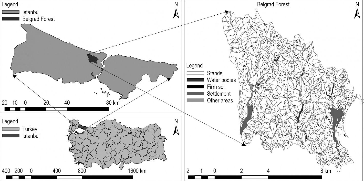
Fig. 1. Location of the case study area: Belgrad Forest in Türkiye
2.2 General Description of MCDA Based Planning Approach
Based on the ecosystem services defined by Kindler (2016), seven ES were identified as important for the study area according to the decisions of 31 stakeholders, as described in Caglayan et al. (2021). The criteria sets were defined to determine the value of each ES. To define these criteria sets, we considered common criteria sets in the literature and the criteria recommended by the experts who have deep knowledge about study area and academic background. For example for the recreation ecosystem service, nine criteria were defined: scenic beauty, elevation, slope, aspect, distance to recreation areas, intensive activity area, accessibility, land cover, and canopy closure (Caglayan et al. 2020). Then, the scores were calculated of each factor of these nine criteria, and normalized using a linear normalization process (Caglayan et al. 2020). The normalized scores of stands were multiplied for each criterion with the main criteria weights. Finally, the multiplied values were calculated and the recreation value of each stand was obtained (Caglayan et al. 2020). In previous studies, the values of other ES were calculated similarly, using distinct criteria. The values are a weighted score between 0 and 1 that each stand receives for each ES.
For the MCDA process, we first defined the criteria sets that may vary the value of ES according to treatment schedules, because the value for each period cannot be computed before having the treatment schedules. Then, the future value of ES was developed for each treatment schedule over a 100-year planning horizon. Then, fifty different treatment schedules were simulated for each stand. Each treatment schedule consists of a reasonable sequence of management activities based on thinning and clear-cutting treatments scheduled over the entire planning horizon. Finally, an optimization model was used to select optimal treatment schedules for each stand to establish a long-term management plan for the forest. The model was applied to six alternative management scenarios representing different approaches for managing the forest. A flow chart (Fig. 2) shows the progress of optimization through these steps of a forest management process.
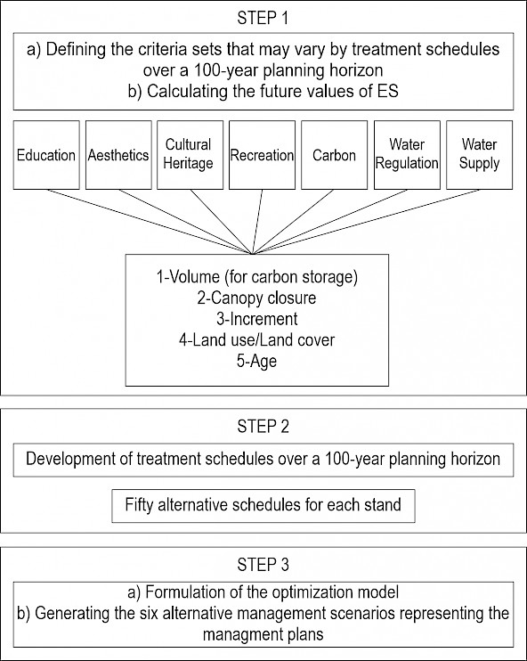
Fig. 2 MCDA-based planning approach based on forest management treatment schedules and valuation to investigate multiple ES
2.2.1 Step 1(a): Defining Criteria Sets that May Vary by Treatment Schedules Over a 100-Year Planning Horizon
For this step, in our previous studies, we defined the predictive criteria sets to the assessment of the initial value of seven ES (e.g., education, aesthetic, cultural heritage, recreation (Caglayan et al. 2020), carbon (Caglayan et al. 2023), water regulation, and water supply). Table 1 illustrates the predictive criteria used to evaluate the value of each ES. The value of some of these criteria may be affected by treatment schedules over a 100-year planning horizon. In our study, 19 criteria are assumed not to be affected by the treatment schedules, while 5 criteria are. The values of these 19 criteria were called fixed parameters. We had no direct measure of the effect of treatment on ecosystem services value and therefore defined management dependent variables as measurable and predictable values that are known to be affected by treatment activities. Five criteria were called management dependent variables. For sub-steps, expert opinions were collected using a questionnaire to determine possible ES for the Belgrad Forest.
In our previous studies, criteria sets were defined for the assessment of the values of seven ES as fixed parameters, and management dependent variables were defined for education, aesthetics, cultural heritage, recreation, carbon, water regulation, and water supply. These parameters and variables were created by using common parameters in the literature and expert opinions for each ES. Finally, the initial value of ES was calculated for each stand (Caglayan et al. 2020, Caglayan et al. 2023). Additionally, there are studies in the literature on calculating the values for education (Nahuelhual et al. 2013), aesthetics (Clay and Daniel 2000, Arriaza et al. 2004), cultural heritage (Hølleland et al. 2017), recreation (Caspersen and Olafsson 2010, Kliskey 2000, Vallecillo et al. 2019), carbon (Baral et al. 2013), water regulation (Guo et al. 2000), and water supply (Villa et al. 2011, Pert et al. 2010, Bagstad et al. 2013) services using different criteria sets. The aim of this study was to calculate the future value of ES. Therefore, the fixed parameters and management dependent variables were defined to evaluate the value of ES for each stand.
Table 1 Predictive criteria sets to evaluate each ES
|
Criteria sets |
Education (k=1) |
Aesthetics (k=2) |
Cultural Heritage (k=3) |
Recreation (k=4) |
Carbon (k=5) |
Water Regulation (k=6) |
Water Supply (k=7) |
|
Fixed parameters (in the model: Bik) |
|||||||
|
Elevation |
|
|
|
x |
|
|
|
|
Slope |
|
|
|
x |
|
x |
x |
|
Aspect |
|
|
|
x |
|
x |
x |
|
Distance to recreational areas |
|
|
|
x |
|
|
|
|
Intensive activity area |
|
|
|
x |
|
|
|
|
Accessibility |
|
|
|
x |
|
|
|
|
Aesthetic |
|
|
|
x |
|
|
|
|
Soil texture |
|
|
|
|
|
x |
x |
|
Precipitation |
|
|
|
|
|
x |
x |
|
Temperature |
|
|
|
|
|
x |
x |
|
Moisture |
|
|
|
|
|
x |
x |
|
Hydrologic |
|
|
|
|
|
x |
x |
|
Water movement |
|
x |
|
x |
|
|
|
|
Water amount |
|
x |
|
x |
|
|
|
|
Negative man-made effects |
|
x |
|
x |
|
|
|
|
Positive man-made effects |
|
x |
|
x |
|
|
|
|
Size of stands |
|
|
|
|
x |
|
|
|
Educational value |
x |
|
|
|
|
|
|
|
Cultural heritage value |
|
|
x |
|
|
|
|
|
Management dependent variables |
|||||||
|
Volume (for carbon storage) (in the model: Vijt) |
|
|
|
|
x |
|
|
|
Increment (in the model: Iijt) |
|
|
|
|
x |
|
|
|
Canopy closure (in the model: CCik) |
|
|
|
x |
|
x |
x |
|
Land cover/Land Use (in the model: LCik) |
|
|
|
x |
x |
x |
x |
|
Age (in the model: Ageijt) |
|
|
|
x |
|
x |
x |
With respect to volume (for carbon storage) (in the model: Vijt) and increment (in the model: Iijt), data for forest growth modelling were extracted from plot-level forest inventory data administered by the GDF. Among the tree species with a yield table are beech (Carus 1998), oak (Eraslan and Evcimen 1967), Turkish red pine (Alemdağ 1962), black pine (Kalıpsız 1963), scotch pine (Alemdağ 1967), fir (Asan 1984), and maritime pine (Özcan 2002). These yield tables were use to calculate the growth parameters. However, there is no a yield table for stone pine, linden, alder, and hornbeam. Therefore, the parameters of the beech yield table were used for linden, alder, and hornbeam. The Turkish pine yield table was also used for stone pine.
The forest growth rate model of the scheduling process used was developed by (Eraslan 1981) and is based on forest inventory data administered by the General Directory of Forestry. The volume of stands is estimated using forest growth and yield models derived from yield tables according to site index and stand age. All stand parameters are calculated at the midpoint of each period. Stands are assumed to develop according to empirical yield tables after final felling. The values of volume development in the current forest are as follows:
 (1)
(1)
 (2)
(2)
Where:
Vij(t+1) future volume after harvest in period t+1
Vijt initial stand volume (m3 ha-1) in period t of treatment schedule j
pjt relative harvest in period t of treatment schedule j
The period length is 20 years.
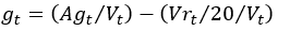
gt growth coefficient in period t for the existing forest
Agt current annual growth (m3 ha-1) in period t in yield table
Vt main stand volume (m3 ha-1) in period t in the yield table
Vrt removed stand volume (m3 ha-1) in period t in yield table.
Since the volume (Vijt) depends on the management, it decreases or increases depending on the treatment program levels in each period. These fluctuations directly affect carbon value. For the optimization model, the volume must be calculated to calculate the carbon value (Table 2).
With respect to canopy closure (in the model: CCik), the Belgrad Forest generally has three canopy closure levels. These are 11–40% (sparse), 41–70% (moderate) and full canopy >71% (dense). Canopy closure and forest dynamics may change after thinnings and final fellings (Tsai et al. 2018). Therefore, in the optimization model, the canopy closure is defined as a variable dependent on management. The model requires an estimate of the canopy closure (CCik) for recreation, water regulation, and water supply values. To protect the level of canopy closure in planning, we assumed that stands would have a relatively dense level canopy after the final felling. As the length of a period is 20 years, and all parameters are calculated according to the middle of the period, young stands will have sufficient growth to have a dense canopy after a previous final felling activity (Table 2). We also assumed that the current level of canopy closure would not be modified after a thinning. If there is a final felling in the treatment schedules, the canopy closure will get the weighted value »e«. Otherwise, »d« represents the weighted value for the current canopy level (Table 2).
With respect to land cover/land use (in the model: LCik) and age (in the model: Ageijt), we classified land use/land cover (LCik) into eleven categories. These are pasture, young conifer stands, middle-aged conifer stands, old conifer stands, young deciduous stands, middle-aged deciduous stands, old deciduous stands, young mixed stands, middle-aged mixed stands, old mixed stands, and irregular stands. Conifer, deciduous- and mixed stands were subdivided into three age classes (Ageijt): Young, 0–60 yrs.; Middle-aged, 61–140 yrs.; and Old, 141+ (Table 2). Irregular stands were tree stands not categorized as coniferous, deciduous, or mixed stands. The land use parameter was correlated with the age parameter in our previous studies. Therefore, the land use parameters modify according to three different age classes (Table 2). We calculated the land cover values of each stand for ES (LCik) that change according to the age of stands for treatment schedules to estimate the land cover value.
2.2.2 Step 1(b): Calculating Future Values of ES
In step 1(b), the values of ES (Sijtk) were calculated after defining management dependent variables in step 1(a) and treatment schedules (step 2). We calculated Sijtk in three different ways because the set of criteria affecting each ES is different. Sijtk values for recreation, water regulation, and water supply are the sum of fixed parameters (Bik), land cover values (LCik), and canopy closure (CCik) of each stand for ES.
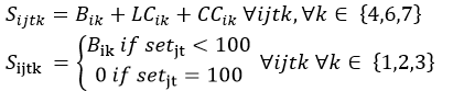 (3)
(3)
The future value of ES of stand i, for treatment schedule j, for ES k recreation (k=4), water regulation (k=6) and water supply (k=7) in period t is the sum of fixed parameters, land cover, and canopy closure (Eqn. 3). Also, the future value of ES of stand i, for treatment schedule j, for ES k education (k=1), aesthetic (k=2) and cultural heritage (k=3) is a fixed parameter or zero in Eqn. 3 because the barren land after the final felling affects these values. Therefore, it was assumed that education, cultural heritage, and aesthetic would only be affected by the final felling. If the treatment schedule includes the final felling, the future value of ES (Sijtk) T
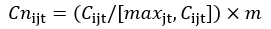
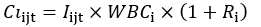
The volume (Vijt), increment (Iijt) and other parameters were used to calculate the future value of ES (Sijtk) for carbon. The amount of annual (Cıijt) and total stored (Cijt) carbon of stands for treatment schedules in periods was calculated using IPCC 2006 equation (Eggleston et al. 2006). Also, the annual and total carbon stored value (Cnijt and Cınijt) was normalized to evaluate the carbon value.
 (4)
(4)
 (5)
(5)
 (6)
(6)
 (7)
(7)
 (8)
(8)
 (9)
(9)
Eqn. 4 represents the carbon storage values of stand i for treatment schedule j, in period t. Eqn. 5 and 7 are for normalization; we have to normalize Cijt and Cıijt due to the value of other ES being normalized. In addition, Clitter is equal to 5.8 tons for C storage in litter, Csoili is equal to 78.0 tons for 1 hectare areas (Tolunay and Çömez 2008). Eqn. 6 represents the annual carbon storage of stand i for treatment schedule j, in period t. In Eqn. 8, we used the coefficient developed by (Tolunay and Çömez 2008) for ground layer carbon storage and carbon litter. Deadwood biomass amounts were estimated as 1% of the aboveground biomass according to (FRA 2015). Since the Forest Planning Regulations have defined that 1 or 2 dead trees must be left per hectare to preserve biodiversity, we accepted deadwood to be about 1% (0.01) of the growing stock per hectare. Eqn. 9 represents the carbon value. Please see Table 2 for the definitions of parameters. Although Step 1b is described prior to Step 2 for methodological clarity, the actual calculation of the future values of ecosystem services ((Sijtk) is performed after the treatment schedules are defined, since these values depend on management-dependent variables that vary by treatment.
Table 2 Definitions of parameters in optimization model data
|
Parameters |
|
Sijtk: future value of stand i, for treatment schedule j, for ES k in period t |
|
Bik: fixed value of stand i for ES k (this is the value of the criteria not affected by the management |
|
LCik: land cover values of stand i for ES k. a, b and c are normalized values
|
|
Ageijt: age of stand i for treatment schedule j, in period t |
|
CCik: canopy closure values of stand i for treatment schedule j. d and e are the normalized values
|
|
setjt: calculated treatment schedule sets for treatment schedule j, in period t |
|
Cijt: carbon storage values of stand i for treatment schedule j, in period t |
|
Cnijt: normalized value of carbon storage stand i for treatment schedule j, in period t |
|
Vijt: volume (m3) produced in the stand i for treatment schedule j, in period t |
|
WBCi: (WD x BEF x CF); WD = wood density (Mg m-3), BEF = biomass expansion factor (non-dimensional). (Tolunay 2019) calculated species-specific biomass expansion factor (BEF) and Wood Density (WD) coefficients for Türkiye. CF is a carbon factor and this value is 0.51 for coniferous, 0.48 for deciduous according to IPCC 2006 (Eggleston et al. 2006), and 0.47 for dead wood |
|
Ri: root to shoot ratio of stand i |
|
Cdeadwoodi: carbon in deadwood biomass of stand i |
|
Clitteri: carbon in litter of stand i |
|
Csoili: carbon in soil of stand i |
|
Iijt: increment of stand i for treatment schedule j, in period t |
|
Cıijt: annual carbon storage of stand i for treatment schedule j, in period t |
|
Cınijt: normalized value of annual carbon storage of stand i for treatment schedule j, in period t |
|
m = 0.635 weight of carbon storage criteria |
|
n = 0.149 weight of carbon increment criteria |
2.2.3 Step 2: Development of Treatment Schedules Over a 100 Year Planning Horizon
This section presents the development of the treatment schedules for the optimization model. Duncker et al. (2012) defined five different forest management approaches: an unmanaged forest nature reserve, low-close-to-nature forestry, medium-combined objective forestry, high-intensive even-aged forestry, intensive-short-rotation forestry. According to this classification, the forestry management approach for Belgrad Forest can be defined as low-close-to-nature forestry. This approach allows harvesting while protecting the forest. Therefore, silvicultural treatment schedules have been determined for fewer operations than are potentially possible in Belgrad Forest. Based on this approach, four alternative management regimes were considered for each stand: (1) No management (NO): in this management regime, no operations are allowed in a forest that might change the nature of the area (Duncker et al. 2012). (2) Final felling (FF): the final harvest may be conducted according to each period but one-time during the planning horizon. (3) Thinning (T): the thinning may be conducted in each period. However, this rate cannot exceed 20% of the growing stock volume. (4) Thinning and Final felling (TFF): TFF represents a management regime where thinning is allowed up to 20% of the the growing stock volume, and the final harvest is set to take place approximately at each period but one-time during the planning period (Table 3). In sum, up to fifty alternative treatment schedules were considered for each stand (Table 3). The future value of ES from step 1(b) is calculated for each stand and fifty treatment schedules are defined in Table 3.
Table 3 Silvicultural treatment schedules (in model: setjt)
|
Treatment schedules |
Management regime |
Period 1 |
Period 2 |
Period 3 |
Period 4 |
Period 5 |
||||||||||
|
Thinning % |
Final felling |
Thinning % |
Final felling |
Thinning % |
Final felling |
Thinning % |
Final felling |
Thinning % |
Final felling |
|||||||
|
20 |
10 |
FF |
20 |
10 |
FF |
20 |
10 |
FF |
20 |
10 |
FF |
20 |
10 |
FF |
||
|
1 |
NO |
|
|
|
|
|
|
|
|
|
|
|
|
|
|
|
|
2 |
FF |
|
|
x |
|
|
|
|
|
|
|
|
|
|
|
|
|
3 |
FF |
|
|
|
|
|
x |
|
|
|
|
|
|
|
|
|
|
4 |
FF |
|
|
|
|
|
|
|
|
x |
|
|
|
|
|
|
|
5 |
FF |
|
|
|
|
|
|
|
|
|
|
|
x |
|
|
|
|
6 |
FF |
|
|
|
|
|
|
|
|
|
|
|
|
|
|
x |
|
7 |
T |
x |
|
|
|
|
|
|
|
|
|
|
|
|
|
|
|
8 |
T |
|
|
|
x |
|
|
|
|
|
|
|
|
|
|
|
|
9 |
T |
|
|
|
|
|
|
x |
|
|
|
|
|
|
|
|
|
10 |
T |
|
|
|
|
|
|
|
|
|
x |
|
|
|
|
|
|
11 |
T |
|
|
|
|
|
|
|
|
|
|
|
|
x |
|
|
|
12 |
TFF |
x |
|
|
|
|
|
|
|
|
|
|
|
|
|
x |
|
13 |
TFF |
|
|
|
x |
|
|
|
|
|
|
|
|
|
|
x |
|
14 |
TFF |
|
|
|
|
|
|
x |
|
|
|
|
|
|
|
x |
|
15 |
TFF |
x |
|
|
|
|
|
|
|
x |
|
|
|
|
|
|
|
16 |
TFF |
|
|
|
x |
|
|
|
|
|
|
|
x |
|
|
|
|
17 |
TFF |
|
|
x |
x |
|
|
|
|
|
|
|
|
|
|
|
|
18 |
TFF |
|
|
|
|
|
x |
x |
|
|
|
|
|
|
|
|
|
19 |
TFF |
|
|
|
|
|
|
|
|
x |
x |
|
|
|
|
|
|
20 |
TFF |
|
|
x |
|
|
|
x |
|
|
|
|
|
|
|
|
|
21 |
TFF |
|
|
|
|
|
x |
|
|
|
x |
|
|
|
|
|
|
22 |
TFF |
|
|
|
|
|
|
|
|
x |
|
|
|
x |
|
|
|
23 |
T |
x |
|
|
x |
|
|
x |
|
|
x |
|
|
x |
|
|
|
24 |
T |
|
x |
|
|
|
|
|
|
|
|
|
|
|
|
|
|
25 |
T |
|
|
|
|
x |
|
|
|
|
|
|
|
|
|
|
|
26 |
T |
|
|
|
|
|
|
|
x |
|
|
|
|
|
|
|
|
27 |
T |
|
|
|
|
|
|
|
|
|
|
x |
|
|
|
|
|
28 |
T |
|
|
|
|
|
|
|
|
|
|
|
|
|
x |
|
|
29 |
TFF |
|
x |
|
|
|
|
|
|
|
|
|
|
|
|
x |
|
30 |
TFF |
|
|
|
|
x |
|
|
|
|
|
|
|
|
|
x |
|
31 |
TFF |
|
|
|
|
|
|
|
x |
|
|
|
|
|
|
x |
|
32 |
TFF |
|
x |
|
|
|
|
|
|
x |
|
|
|
|
|
|
|
33 |
TFF |
|
|
|
|
x |
|
|
|
|
|
|
x |
|
|
|
|
34 |
TFF |
|
|
x |
|
x |
|
|
|
|
|
|
|
|
|
|
|
35 |
TFF |
|
|
|
|
|
x |
|
x |
|
|
|
|
|
|
|
|
36 |
TFF |
|
|
|
|
|
|
|
|
x |
|
x |
|
|
|
|
|
37 |
TFF |
|
|
x |
|
|
|
|
x |
|
|
|
|
|
|
|
|
38 |
TFF |
|
|
|
|
|
x |
|
|
|
|
x |
|
|
|
|
|
39 |
TFF |
|
|
|
|
|
|
|
|
x |
|
|
|
|
x |
|
|
40 |
T |
|
x |
|
|
x |
|
|
x |
|
|
x |
|
|
x |
|
|
41 |
TFF |
x |
|
|
|
|
|
|
x |
|
|
|
|
|
|
x |
|
42 |
TFF |
|
x |
|
|
|
|
x |
|
|
|
|
|
|
|
x |
|
43 |
TFF |
|
|
x |
|
|
|
x |
|
|
|
|
|
|
x |
|
|
44 |
TFF |
|
|
x |
|
|
|
|
x |
|
|
|
|
x |
|
|
|
45 |
TFF |
x |
|
|
|
x |
|
|
|
x |
|
|
|
|
|
|
|
46 |
TFF |
|
|
|
x |
|
|
|
x |
|
|
|
x |
|
|
|
|
47 |
TFF |
|
|
|
|
|
|
x |
|
|
|
x |
|
|
|
x |
|
48 |
TFF |
|
x |
|
x |
|
|
|
x |
|
x |
|
|
|
x |
|
|
49 |
TFF |
x |
|
|
|
x |
|
x |
|
|
|
x |
|
x |
|
|
|
50 |
TFF |
x |
|
|
x |
|
|
|
x |
|
|
x |
|
|
|
x |
2.2.4 Step 3(a): Formulation of Optimization Model
The objective function of the planning problem is to maximize a utility function value that can include the future value of education, aesthetic, cultural heritage, recreation, carbon, water supply, and water regulation. There were also some management activities and assumptions for ES planning approaches. The general planning problem consists of selecting one scenario (of the 50 treatment schedules) for each stand in the landscape so that the total weighted utility from a set of ES over the entire planning horizon is maximized. The calculations were made by using the AIMMS optimizer. The included ES are education, aesthetics, cultural heritage, recreation, carbon, water supply, and water regulation. Timber production is not identified as an ES. However, it was included as a constraint for a minimum harvest level each period. In addition, other constraints could be included. The mathematical formulation of the problem is as follows. Please see Table 4 for the definitions of sets, parameters, and decision variables. SDG was determined according to the expert opinion for ES in our previous study. These are Life on Land, Clean Water & Sanitation, Good Health & Well-Being, Climate Action, and Decent Work & Economic Growth (Table 4). The Stakeholder groups weighted the SDG. Finally, they associated the SDG and ES (in the model; wp).
Table 4 Definitions for mixed integer programming formulation
|
Sets and Indices |
|
i, i1 : stands (i = 1,…,I, i1 = 1,…I) |
|
j, set of treatment schedules (j = 1,…J) |
|
t, set of all periods (t = 1,..T) |
|
k: set of ES (k = 1,…K) k = 1 is education, k = 2 is aesthetics, k = 3 is cultural heritage, k = 4 is recreation, k = 5 carbon, k = 6 is water regulation, and k = 7 is water supply |
|
p: sustainable developments goals (SDG) (p = 1, ….P) p = 1 is Life on Land, p = 2 is Clean Water & Sanitation, p = 3 is Good Health & Well-Being, p = 4 is Climate Action, and p = 5 is Decent Work & Economic Growth |
|
N: set of neighbor stands, N = (i, i1) | i and i1 are neighbors |
|
Parameters |
|
ai: area (ha) of stand i |
|
Wp: weights of SDG p ( |
|
hijt: harvested volume of stand i for treatment schedule j, in period t |
|
tijt: thinning volume of stand i for treatment schedule j, in period t |
|
V: total harvest demand, m3 |
|
Dkp: level of support for ES (k) and SDG (p) contributions |
|
Variables |
|
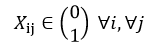
Xij: binary decision variable indicating the assignment of treatment schedule j to stand i
|
|
U: utility function value |
|
Mijt: variable indicating if treatment j will be chosen for stand i or not (0–1) |
|
Ht: total harvested volume in period t |
|
Tt: total thinning volume in period t |
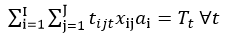
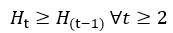
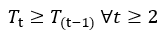
The objective function is presented in Eqn. 11. Eqn. 12 limits treatment activity in a unit to occur once at most. In Eqn. 13, i and i₁ represent neighboring stands within the adjacency set N. The parameter maxadjacency denotes the maximum number of adjacent stands that can be harvested in the same period. Its value is scenario-dependent and is defined in Table 5. Eqn. 14 is the harvested volume of each period. Eqn. 15 is the thinning volume of each period. In Eqn. 16, harvest volume constraints limited the ranges of the scheduled volume during each period. The volume control equations (Eqn. 17) impose that timber volume harvested in t period will be more from t-1 periods. The thinning volume control equations (Eqn. 18) impose that thinning volume harvested in t. period will be more from t-1 periods. Also, Eqn. 19 limits the total harvest level from GDF for the harvest demand. The future value of ES control equations (Eqn. 20) imposes that these values in t period will be more from t-1 periods.
 (11)
(11)
Subject to;
 (12)
(12)
 (13)
(13)
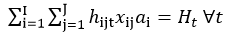 (14)
(14)
 (15)
(15)
 (16)
(16)
 (17)
(17)
 (18)
(18)
 (19)
(19)
 (20)
(20)
2.2.5 Step 3(b): Generating Six Alternative Management Scenarios Representing Management Plans
By including four different constraints, six alternative management scenarios were developed. The constraints were associated with harvested volume (the sum of thinning and final felling) and included an adjacency (Eqn. 13), wood flow (Eqn. 17), thinning volume (Eqn. 18), harvest demand (Eqn. 19), and the future value of ES (Eqn. 20). Eqns. 17–20 represent non-declining constraints, ensuring that harvested volumes and ES values either remain constant or increase from one period to the next, reflecting sustainable forest management goals. Due to the »low close to nature forestry« approach, the wood flow constraint was added to control the wood production, and the adjacency constraint was added so as not to exceed the maximum opening area. A harvest demand constraint was also added to meet the demands of the GDF. Finally, a constraint was added on the future value of ES as in our opinion these values should increase in every period. In this context, six alternative management scenarios were developed (Table 5). In scenario 1, forest management is focused on maximizing the total utility by contributing to the higher harvest and the future value of ES in forests. It was designed to describe management approaches aimed towards nature conservation and increased the constraints to minimize the harvest in scenario 2. Scenario 3 was designed to limit only by the constraints the increase of future ES in each period. In scenario 4, the nature conservation approach was adopted to reduce harvest intensity.
In the previous GDF forest management plans, it was suggested that 7471 m3 of the average annual final harvest and 11,413 m3 of the annual thinning volume could be obtained from this forest. Therefore, in the 20-year time periods, the final harvest level is estimated to be about 150,000 m3 and the thinning harvest about 220,000 m3. Consequently, it is expected that 370,000 m3 of the total harvest will be scheduled during the entire time horizon. However, these harvest amounts contradict with the planning approach of forest ES. For this reason, Scenario 5 was developed to indicate that these harvest amounts in the GDF management plans may be too high. Designed according to the existing harvest level based on management plans, Scenario 5 allows the total final harvest to range between 120,000 m3 and 150,000 m3. Here too, the total thinning harvest was not considered. Scenario 6 was designed according to the nature conservation approach by narrowing the restrictions defined in Strategy 5. Therefore, the total final harvest was allowed to range between 80,000 m3 and 100,000 m3.
Table 5 Six alternative management scenarios
|
Scenario number |
Constraints |
Objective Level |
|
1 |
No wood flow constraint |
Maximization of the future value of ES when there are no constraints. Thin only on a small scale. Let the forest grow old |
|
No adjacency constraint |
||
|
No future value of ES constraint |
||
|
No harvest demand |
||
|
2 |
Wood flow constraint |
Maximization of the future value of ES in case regeneration of four adjacent stands at most, these values in period t will be greater than in period t-1, thinning and harvest volumes in period t will be greater than in period t-1. Harvest volume in period t will be greater than 17,000 m3 |
|
Adjacency constraint |
||
|
Future value of ES constraint |
||
|
Harvest demand |
||
|
3 |
No wood flow constraint |
Maximization of the future value of ES with the constraint that these values in period t will be greater than in period t-1 |
|
No adjacency constraint |
||
|
Future value of ES constraint |
||
|
No harvest demand |
||
|
4 |
Wood flow constraint |
Maximization of the future value of ES in case of regeneration of four adjacent stands at most, and increase the harvest volume during each subsequent period. Also, harvest volume in period t will be greater than 20,000 m3 |
|
Adjacency constraint |
||
|
Future value of ES constraint |
||
|
Harvest demand |
||
|
5 |
Wood flow constraint |
Maximization of ES utility in case of regeneration of seven adjacent stands at most, and increase the harvest volume during each subsequent period. Also, harvest in period t will be between 120,000 and 150,000 m3 |
|
Adjacency constraint |
||
|
Future value of ES constraint |
||
|
Harvest demand |
||
|
6 |
Wood flow constraint |
Maximization of ES utility in case of regeneration of six adjacent stands at most, and increase the harvest volume during each subsequent period. Also, harvest in period t will be between 80,000 and 100,000 m3 |
|
Adjacency constraint |
||
|
Future value of ES constraint |
||
|
Harvest demand |
2.3 Software Used
Forest inventory data related to the Belgrad Forest was used. In the scheduling process, a mixed-integer linear programming model was used to select scenarios and maximize the value of the objective function during the planning horizon. ArcMap, R studio, and AIMMS programs were used to obtain various spatial data and solve the mathematical model, respectively. All experiments have been conducted on a personal computer with 3.40 GHz CPU and 8 GB of RAM. The time required to generate a solution to the problem formulations using CPlex 12.9 was an average of 287.903 sec.; from Scenario 1 to Scenario 6: 13.2, 903.6, 32.8, 69.97, 181.31, and 526.53 sec, respectively.
3. Results
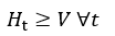
The results of the optimization process associated with ES management approaches include the corresponding value of the seven ES in addition to the amounts of timber scheduled for harvest. At the end of planning horizon, a total of 1,433,335.7 m³ of wood was scheduled for harvest in Scenario 1, 85,542.9 m³ in Scenario 2, 1,424,706.5 m³ in Scenario 3, 100,027.7 m³ in Scenario 4, 623,663.9 m³ in Scenario 5, and 400,036.0 m³ in Scenario 6. More timber was scheduled for harvest in Scenario 1 than the other alternatives, and it also had the highest objective function value. In Fig. 3, the stacked bar chart is created for each scenario divided into parts that are proportional to thinning and final felling level percentage. In the scenarios, the majority of the harvest is obtained from thinnings. In Scenarios 2 and 6, the thinning and final harvest volumes are approximately equal to each other.
In Scenario 2, all constraints are active, which reduced the objective function value of the resulting plan. With Scenario 2, the number of neighboring stands is controlled during harvest, while at the same time, the scheduled harvest is constrained. As a result, Scenario 2 shows that the future value of ES can be increased as long as the harvest amount is not reduced below 17,000 m3.
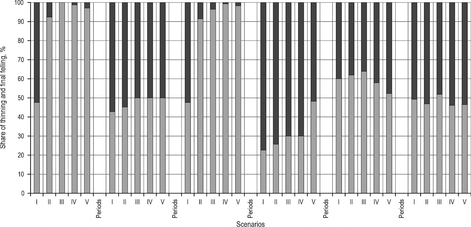
Fig. 3 Percentage distribution of thinning and final felling volume (from Scenario 1 to Scenario 6, respectively)
In Fig. 4, the line chart illustrates estimated changes for each ES over time. The water regulation service has a higher ES than water supply, carbon, cultural heritage, recreation, education, and aesthetic ES. There is not much fluctuation in the values of water supply, water regulation, cultural heritage, recreation, aesthetics, and education services according to the results (Fig. 4), yet the carbon ES had the highest fluctuation between time periods and scenarios.
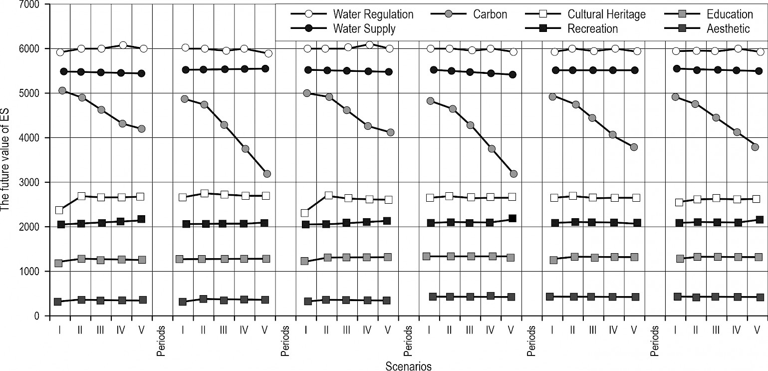
Fig. 4 Future value of ES according to scenarios (from Scenario 1 to Scenario 6, respectively)
According to Scenarios 1 and 3, different scheduled timber harvest levels are obtained in each period (Fig. 5a). Scenarios 2, 4, and 6 show that scheduled harvest levels are approximately equal in each time period. The highest fluctuations in scheduled harvest levels across a time horizon are seen in Scenarios 1 and 3. We found total carbon storage of 4,718,974.6 m3 for Scenario 1, 6,574,804.2 m3 for Scenario 2, 4,725,098.4 m3 for Scenario 3, 6,572,149.3 m3 for Scenario 4, 5,951,327.4 m3 for Scenario 5, and 6,251,265.1 m3 for Scenario 6, respectively (Fig. 5b). The results show that, as the scheduled harvest level increases, the amount of carbon storage decreases (Fig. 5b), thus the amount of carbon stored is inversely proportional to the harvest level. As each scenario emphasizes the attainment of different goals, through the constraints that are imposed, the timing and placement of the proposed scheduled activities across the landscape vary considerably (Fig. 6).
Fig. 5 Harvest level (m3) according to scenarios (a), and amount of carbon storage (m3 ha-1) according to scenarios (b)
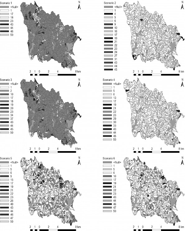
Fig. 6 Maps showing spatial distribution of treatment schedules for six alternative management scenarios (Colors represent the fifty treatment schedules)
4. Discussion
In the present study, a new spatially explicit approach has been developed for the evaluation of forest management scenarios to maximize utility value based on seven ES. This approach was designed especially for our study in the Belgrad Forest, Türkiye, where the functional planning approach began in 2008, yet the design of the model is novel and potentially applicable in other forested areas of the world. In addition to the assessment of ESs, the characteristic of this approach is that it can assist in building the tactical plan for a landscape while ensuring that long-term strategic issues are acknowledged. The planning process may be able to improve ecosystem management by providing a set of optimal solutions to guide forest managers using the problem formulation we described. While the acknowledgement of ecosystem service values is relatively simple compared to elegant works that provide more detailed analyses, simplications of functional relationships between forest management activities and outcomes of interest in forest planning are sometimes necessary when the science is still developing. The progression of work related to the incorporation of wildfire effects into forest harvest scheduling is a good example (Bettinger 2010). Nonetheless, with the approach we described, one can study the changes that are expected to occur with respect to the ES of importance in any study area. Furthermore, one can design various scenarios for multi-objective forest management, analyze alternative scenarios, and obtain high quality forest management solutions that can be visualized in a variety of ways to inform decision makers.
In this study, the values of seven ES were considered, and therefore the future values of ES were integrated into the forest management planning process with quantitative methods to achieve sustainable forest management initiatives (Baskent et al. 2008). Optimization studies on forest management are often focused on maximizing the net present value (NPV) or some other economic or commodity production goal (Robinson et al. 2016). However, this study aimed to maximize future resource utility, placing financial objectives as secondary to the combined future value of ES. While early models often used simplified relationships, recent literature (e.g., Baskent and Balci 2024) shows a clear trend towards more complex, flexible, and globally relevant models. The inclusion of multiple metrics into the assessment of utility thus requires additional, robust ways to assess current and future values of those metrics. Further, a functional relationship between the management decisions (thinnings, final harvests, doing nothing) and the outcomes or levels of these metrics needs to be clear.
In general, our results show that, when there are relatively few constraints (Scenario 1), a wide fluctuation of scheduled harvest levels may occur across the time periods of the time horizon for this forested landscape. This can be a very undesirable outcome in terms of forest management, yet it is based on the current condition of the forest and assumptions about future growth. Similar problems may be encountered by other forests around the world. Scenario 3 was designed to be limited only by the constraint where the future value of ES needed to increase in each period. However, in Scenario 3 we have achieved results almost comparable to Scenario 1. Consequently, the constraint of increasing the future value of ES in each period does not affect the model outcomes very much. For example, if treatment schedule 23 is selected, which implies a 20% thinning in each period, both the highest value of ES and the utility value of the objective function should increase.
Our results show that forest management mainly directed at nature conservation (Scenario 2) decreases the scheduled harvest level by about 94% compared to Scenario 1. In addition, Scenario 4 also represents a nature conversation management approach. Despite similar trends of nature conservation for Scenario 2 in comparison with Scenario 4, we showed that the scheduled harvest level of Scenario 4 increased by about 14% from Scenario 2. A forest management approach mainly geared towards increasingly maximizing the future value of ES from each period (Scenario 3) interestingly almost equals the scheduled harvest level of Scenario 1. Scenario 5 was designed according to the final harvest level limits estimated by the GDF for this landscape. The total scheduled thinning harvest was not taken into consideration since the total harvest (thinning and final felling) will be 370,000 m3 in the 20-year period. Consequently, this amount will be about 1,850,000 m3 over a 100-year planning horizon. However, since this amount is too large even for Scenario 1, where all the constraints have been loosened, we have only considered the final harvest level constraint. If scenarios are determined according to harvest levels estimated by the GDF, this scenario will be far from the nature conservation management approach. In the next national planning period, the GDF might examine reducing the total scheduled harvest levels to amounts lower than previous plans suggest, to potentially conserve the future value of ES. By applying this integrated optimization approach, managers can better evaluate trade-offs among multiple ES and adjust management strategies to enhance long-term ecosystem resilience and value, fostering sustainable forest management aligned with both ecological and socio-economic objectives.
While our approach offers a systematic method for integrating multiple ES into forest planning, it should be noted that forest management contexts vary widely. This framework provides a flexible foundation that managers can adapt to specific local conditions, stakeholder priorities, and governance structures. While Bottalico et al. (2016) show that harvest intensity and frequency may affect the attainment of several ES, in our study the harvest intensity only affected the carbon ES. This is because scheduled harvest volume is only used as a variable when estimating the carbon ES value, and not when assessing the other ES values. Consequently, as the value of the carbon ES changed, only the scheduled harvested volume changed noticeably, according to scenarios and treatment schedules. While treatment schedules also affect management-dependent variables such as canopy closure or age, which influence other ES, these variables were not dynamically linked to those ES in our model, and therefore their values remained largely constant. Therefore, if the value of a forest ES will be used as a parameter for strategic forest planning, the volume of carbon sequestered should be included as a criterion in the functional relationships that connect management activities to the attainment of ES values.
Recreation, water regulation, and water supply are all associated with forest canopy cover. In our analysis, it was assumed that a harvested stand would immediately be restocked, and that it will have a closed canopy after 10 years, which may be a shortcoming of our analyses. Hence the assumptions made in this study extend their impact over other characteristics of the forest, as modeled. This reinforces the need for acquiring or developing strong, valid assumptions regarding forest dynamics. Consequently, if future projections of forest change are uncertain and beyond the interest of analysts and policymakers, a shorter time horizon should be adopted in ES management modeling studies.
In our model, the inclusion of the land cover variable aimed to capture broader forest dynamics, including tree species composition and species mixtures, which extend beyond age dependency. While some land cover classes may be partially influenced by stand age, this variable was not solely defined by age but also by spatial and structural characteristics relevant to ecosystem service evaluation. Additionally, stand age was incorporated as a separate variable to address growth dynamics and treatment responses specific to forest management planning. This dual consideration ensures that the model captures both general forest attributes and management-specific processes, providing a more robust framework for evaluating ecosystem services. Future studies could enhance this framework by incorporating advanced methodologies to refine these relationships and better represent the multifaceted nature of forest ecosystems.
Stopping wood production to protect the carbon pool does not mean that you guarantee protection (Hoover and Stout 2007, Moreno-Fernández et al. 2015, Paradis et al. 2019). For example, as a result of the aging of forests without managing may increase large-scale different abiotic and biotic damage, thus forest carbon stocks may decrease (Seidl et al. 2017). However, others have shown (Kucuker 2019) that, when total harvest intensity decreases, carbon sequestration can increase. These conclusions may be forest-specific, as we have shown that carbon sequestration in the forest can be increased or decreased with various silvicultural treatments. Therefore, it cannot be said that in all cases the carbon capture potential can be increased when forests are not managed. The results regarding the increase or decrease of carbon capture potential when a forest is managed can only be revealed by exploring alternative planning strategies. As Cook-Patton et al. (2020) state, additional studies are needed to characterize the climate change mitigation potential of alternative management strategies.
5. Conclusions
This study employed the future value of ES that a forest could provide to help evaluate several different management scenarios. Ecosystem service values were estimated using fixed parameters and management dependent variables. Fifty potential treatment schedules were designed for each stand. This information was used in an optimization process that maximized the utility value of ES, using weights related to SDG, over a 100-year planning horizon. The results show that our approach can be used to produce the optimal future ES values for a forested landscape within a long-term forest planning structure. However, among the management dependent variables, standing forest volume and growth increment directly affect carbon values, while forest age, land use, and canopy closure affect the value of other ES.
Among the ES modeled, carbon showed the highest fluctuations due to its direct link with scheduled harvest volume and growth increment. Other ES remained relatively stable because their values were derived primarily from fixed parameters and were not dynamically linked to changing variables such as age or canopy. While forest age can influence certain ES, it was not functionally connected to those ES in the model due to the lack of empirical data or established relationships for such linkages. Future studies could explore how age-related dynamics might affect additional ES to enhance model sensitivity.
By integrating ES into a mathematical planning process, this process can be described as an extended harvest scheduling problem. In this endeavor, we found that the development of suitability value-effective management strategies for securing forest ES values in future stand developments was possible while also achieving other goals and while also being constrained by operational considerations. This integrated optimization framework supports forest managers and policymakers in aligning ecological objectives with societal priorities, fostering sustainable strategies for resilient forest landscapes. While our study started from a local perspective, the flexibility of the proposed optimization framework holds promise for broader applications. By adjusting input parameters and criteria, managers worldwide could apply this approach to their unique ecological and socio-economic contexts. Furthermore, by incrementally refining ES valuation methods and incorporating emerging insights from global research, this approach can evolve to support more diverse forest management contexts. The new work presented in this study contributes to ongoing debates on general relationships between commodity production benefits and the future value of ES associated with forest management scenarios. This study also enables decision-makers to better guide forest management strategies in the future.
Acknowledgements
Funding: This work was supported by the Scientific and Technological Research Council of Türkiye (TÜBİTAK) (project 2214-A) [Applied number: 1059B141800151). We are grateful to the TÜBİTAK for funding.
6. References
Alemdağ, Ş., 1962: Türkiye’deki kızılçam ormanlarının gelisimi, hasılatı veamenajman esasları. Orman Araştırma Enstitüsü 11: Istanbul, Turkey.
Alemdağ, Ş., 1967: Türkiyede sarıçam ormanlarının kuruluşu, verim gücü ve bu ormanların işletilmesinde takip edilecek essaslar. Orman Arastırma Enstitüsü Teknik bül: 4. Istanbul, Turkey.
Arriaza, M., Cañas-Ortega, J.F., Cañas-Madueño, J.A., Ruiz-Aviles, P., 2004: Assessing the visual quality of rural landscapes. Landsc Urban Plan 69(1): 115–125. https://doi.org/10.1016/j.landurbplan.2003.10.029
Asan, Ü., 1984: Kazdağı Göknarı (Abies equi-trojani Aschers, et Sinten.) ormanlarının hasılat ve amenajman esasları üzerine araştırmalar. İÜ Orman Fakültesi, Istanbul, Turkey, Yayını, 365 p.
Bagstad, K.J., Semmens, D.J., Winthrop, R., 2013: Comparing approaches to spatially explicit ecosystem service modeling: A case study from the San Pedro River, Arizona. Ecosyst Serv 5: 40–50. https://doi.org/10.1016/j.ecoser.2013.07.007
Bagstad, K.J., Villa, F., Johnson, G.W., Voigt, B., 2011: ARIES (Artificial Intelligence for Ecosystem Services): A guide to models and data, version 1.0. The ARIES Consortium. ARIES report series no. 1.
Baral, H., Keenan, R.J., Fox, J.C., Stork, N., 2013: Spatial assessment of ecosystem goods and services in complex production landscapes: A case study from south-eastern Australia. Ecol Complex 13: 35–45. https://doi.org/10.1016/j.ecocom.2012.11.001
Başkent, E.Z., 2018: A review of the development of the multiple use forest management planning concept. Int For Rev 20(3): 296–313. https://doi.org/10.1505/146554818824063023
Baskent, E.Z., Borges, J.G., Kašpar, J., Tahri, M., 2020: A design for addressing multiple ecosystem services in forest management planning. Forests 11(10): 1108. https://doi.org/10.3390/f11101108
Baskent, E.Z., Keles, S., Yolasigmaz, H.A., 2008: Comparing multipurpose forest management with timber management, incorporating timber, carbon and oxygen values: A case study. Scand J For Res 23(2): 105–120. https://doi.org/10.1080/02827580701803536
Başkent, E.Z., Balci, H., 2024: A priory allocation of ecosystem services to forest stands in a forest management context considering scientific suitability, stakeholder engagement and sustainability concept with multi-criteria decision analysis (MCDA) technique: A case study in Turkey. Journal of Environmental Management 369: 122230. https://doi.org/10.1016/j.jenvman.2024.122230
Bennett, E.M., Peterson, G.D., Gordon, L.J., 2009: Understanding relationships among multiple ecosystem services. Ecol Lett 12(12): 1394–1404. https://doi.org/10.1111/j.1461-0248.2009.01387.x
Bettinger, P., 2010: An overview of methods for incorporating wildfires into forest planning models. Math Comp Forestry & Nat Res Sci 2(1): 43–52.
Bottalico, F., Pesola, L., Vizzarri, M., Antonello, L., Barbati, A., Chirici, G., Corona, P., Cullotta, S., Garfi, V., Giannico, V., Lafortezza, R., Lombardi, F., Marchetti, M., Nocentini, S., Riccioli, F., Travaglini, D., Sallustio, L., 2016: Modeling the influence of alternative forest management scenarios on wood production and carbon storage: A case study in the Mediterranean region. Environ Res 144(B): 72–87. https://doi.org/10.1016/j.envres.2015.10.025
Boumans, R., Costanza, R., 2007: The multiscale integrated Earth Systems model (MIMES): the dynamics, modeling and valuation of ecosystem services. Issues Glob Water Syst Res 2(2): 10–11
Cademus, R., Escobedo, F.J., McLaughlin, D., Abd-Elrahman, A., 2014: Analyzing trade-offs, synergies, and drivers among timber production, carbon sequestration, and water yield in Pinus elliotii forests in Southeastern USA. Forests 5(6): 1409–1431. https://doi.org/10.3390/f5061409
Caglayan, İ., Yeşil, A., Cieszewski, C., Kilic Gul, F., Kabak, Ö., 2020: Mapping of recreation suitability in the Belgrad Forest Stands. Appl Geogr 116: 102153. https://doi.org/10.1016/j.apgeog.2020.102153
Caglayan, İ., Yeşil, A., Kabak, Ö., Bettinger, P., 2021: A decision making approach for assignment of ecosystem services to forest management units: A case study in northwest Turkey. Ecol Indic 121: 107056. https://doi.org/10.1016/j.ecolind.2020.107056
Caglayan, I., Yeşil, A., Tolunay, D., Petersson, H., 2023: Carbon suitability mapping for forest management plan decisions: The Case of Belgrad Forest (Istanbul). Environmental Modeling & Assessment 28(2): 175–188. https://doi.org/10.1007/s10666-022-09856-z
Carus, S., 1998: Aynı Yaslı Doğu Kayını (Fagus orientalis Lipsky.) OrmanlarındaArtım ve Büyüme. İstanbul University, Istanbul, Turkey.
Caspersen, O.H., Olafsson, A.S., 2010: Recreational mapping and planning for enlargement of the green structure in greater Copenhagen. Urban For Urban Green 9(2): 101–112. https://doi.org/10.1016/j.ufug.2009.06.007
Chan, K.M.A., Shaw, M.R., Cameron, D.R., Underwood, E.C., Daily, G.C., 2006: Conservation planning for ecosystem services. PLoS Biol 4(11): 2138–2152. https://doi.org/10.1371/journal.pbio.0040379
Clay, G.R., Daniel, T.C., 2000: Scenic landscape assessment: The effects of land management jurisdiction on public perception of scenic beauty. Landsc Urban Plan 49(1-2): 1–13. https://doi.org/10.1016/S0169-2046(00)00055-4
Coelho Junior,M.G., Biju, B.P., Silva Neto, E.C. 2020: Improving the management effectiveness and decision-making by stakeholders’ perspectives: A case study in a protected area from the Brazilian Atlantic Forest. J Environ Manage 272:111083. https://doi.org/10.1016/j.jenvman.2020.111083
Cook-Patton, S.C., Leavitt, S.M., Gibbs, D., Harris, N.L., Lister, K., Anderson-Teixeira, K.J., Briggs, R.D., Chazdon, R.L., Crowther, T.W., Ellis, P.W., Griscom, H.P, Herrmann, V., Holl, K.D., Houghton, R.A., Larrosa, C., Lomax, G., Lucas, R., Madsen, P., Malhi, Y., Paquette, A., Parker, J.D., Paul, K., Routh, D., Roxburgh, S., Saatchi, S., van den Hoogen, J., Walker, W.S., Wheeler, C.E., Wood, S.A., Xu, L., Griscom, B.W., 2020: Mapping carbon accumulation potential from global natural forest regrowth. Nature 585(7826): 545–550. https://doi.org/10.1038/s41586-020-2686-x
Costanza, R., D’Arge, R., De Groot, R., Farber, S., Grasso, M., Hannon, B., Limburg, K., Naeem, S., ONeill, R.V., Paruelo, J., Raskin, R.G., Sutton, P., van den Belt, M., 1997: The value of the world’s ecosystem services and natural capital. Nature 387(6630): 253–260. https://doi.org/10.1038/387253a0
Dong, L., Lin, X., Bettinger, P., Liu, Z.: 2024: How to maximize the joint benefits of timber production and carbon sequestration for rural areas? A case study of larch plantations in northeast China. Carbon Balance and Management 19(1): 24. https://doi.org/10.1186/s13021-024-00271-3
Duncker, P., Barreiro, S., Hengeveld, G., Lind, T., 2012: Classification of forest management approaches: A new conceptual framework and its applicability to European forestry. Ecol Soc 17(4): 51. https://doi.org/10.5751/ES-05262-170451
Eggleston, S., Buendia, L., Miwa, K., 2006: IPCC guidelines for national greenhouse gas inventories. Institute for Global Environmental Strategies, Yokohama, Japan.
Egoh, B., Drakou, E., Dunbar, M.B., Maes, J., Willemen, L., 2012: Indicators for mapping ecosystem services : a review. Technical Report EUR25456EN. European Commission, Joint Research Centre (JRC), Luxembourg. https://doi.org/10.2788/41823
Eraslan, İ., 1981: Aynı yaşlı ormanların optimal kuruluşlara götürülmesinde kullanılabilecek artım yüzdeleri simulasyon yöntemi. J Fac For Istanbul Univ No. 2110/2:38
Eraslan, İ., Evcimen, B.S., 1967: Trakya’ daki mese ormanlarının hacim ve hasılatı hakkında tamamlayıcı arastırmalar. İÜ Orman Fakültesi, Istanbul, Turkey. Dergisi SeriA.
FRA., 2015: Turkey-Global Forest Resources Assesment-Country Report. Rome
Garcia-Gonzalo, J., Bushenkov, V., McDill, M.E., Borges, J.G., 2015: A decision support system for assessing trade-offs between ecosystem management goals: An application in portugal. Forests 6(1): 65–87. https://doi.org/10.3390/f6010065
Geneletti, D., 2011: Reasons and options for integrating ecosystem services in strategic environmental assessment of spatial planning. Int J Biodivers Sci Ecosyst Serv Manag 7(3): 143–149. https://doi.org/10.1080/21513732.2011.617711
Grêt-Regamey, A., Weibel, B., Kienast, F., Rabe, S.E., Zulian, G., 2015: A tiered approach for mapping ecosystem services. Ecosyst Serv 13: 16–27. https://doi.org/10.1016/j.ecoser.2014.10.008
Guo, Z., Xiao, X., Li, D., 2000: An assessment of ecosystem services: Water flow regulation and hydroelectric power production. Ecol Appl 10(3): 925–936. https://doi.org/10.1890/1051-0761(2000)010[0925:AAOESW]2.0.CO;2
Haara, A., Pykäläinen, J., Tolvanen, A., Kurttila, M., 2018: Use of interactive data visualization in multi-objective forest planning. J Environ Manage 210: 71–86. https://doi.org/10.1016/j.jenvman.2018.01.002
Haines-Young, R., Potschin, M., 2012: Common International Classification of Ecosystem Services (CICES, Version 4.1) Centre for Environmental Management, School of Geography, University of Nottingham, Nottingham, UK.
Hølleland, H., Skrede, J., Holmgaard, S.B., 2017: Cultural heritage and ecosystem services: A literature review. Conserv Manag Archaeol Sites 19(3): 210–237. https://doi.org/10.1080/13505033.2017.1342069
Hoover, C., Stout, S., 2007: The carbon consequences of thinning techniques: Stand structure makes a difference. J For 105(5): 266–270. https://doi.org/10.1093/jof/105.5.266
Hu, H., Fu, B., Lü, Y., Zheng, Z., 2015: SAORES: a spatially explicit assessment and optimization tool for regional ecosystem services. Landsc Ecol 30: 547–560. https://doi.org/10.1007/s10980-014-0126-8
ITTO, 2002: ITTO guidelines for the restoration , management and rehabilitation of degraded and secondary tropical forests. International Tropical Timber Organization, Yokohama, Japan. ITTO Policy Development Series No 13.
Jakeman, A.J., Letcher, R.A., Norton, J.P., 2006: Ten iterative steps in development and evaluation of environmental models. Environ Model Softw 21(5): 602–614. https://doi.org/10.1016/j.envsoft.2006.01.004
Juerges, N., Arts, B., Masiero, M., Baskent, E.Z., Borges, J.G., Brodrechtova, Y., Brukas, V., Canadas, M.J., Carvalho, P.O., Corradini, G., Corrigan, E., Felton, A., Hoogstra-Klein, M., Krott, M., van Laar, J., Lodin, I., Lundholm, A., Makrickiene, E., Marques, M., Mendes, A., Pivoriunas, N., 2020: Integrating ecosystem services in power analysis in forest governance: A comparison across nine European countries. For Policy Econ 121: 102317. https://doi.org/10.1016/j.forpol.2020.102317
Kalıpsız, A., 1963: Türkiye’de Karaçam (Pinus nigra Arnold) mescerelerinin tabii bünyesi ve verim kudreti üzerine arastırmalar. Sıra No: 3 Istanbul, Turkey.
Kindler, E., 2016: A comparison of the concepts: Ecosystem services and forest functions to improve interdisciplinary exchange. For. Policy Econ. 67: 52-59. https://doi.org/ 10.1016/j.forpol.2016.03.011
Kliskey, A.D., 2000: Recreation terrain suitability mapping: A spatially explicit methodology for determining recreation potential for resource use assessment. Landsc Urban Plan 52(1): 33–43. https://doi.org/10.1016/S0169-2046(00)00111-0
Köchli, D.A., Brang, P., 2005: Simulating effects of forest management on selected public forest goods and services: A case study. For Ecol Manage 209(1–2): 57–68. https://doi.org/10.1016/j.foreco.2005.01.009
Kucuker, D.M., 2019: Analyzing the effects of various forest management strategies and carbon prices on carbon dynamics in western Turkey. J Environ Manage 249: 109356. https://doi.org/https://doi.org/10.1016/j.jenvman.2019.109356
Liu, J., Dietz, T., Carpenter, S.R., Alberti, M., Folke, C., Moran, E., Pell, A.N., Deadman, P., Kratz, T., Lubchenco, J., Ostrom, E., Ouyang, Z., Provencher, W., Redman, C.L., Schneider, Sh., Taylor, W., 2007: Complexity of coupled human and natural systems. Science 317(5844): 1513–1516. https://doi.org/10.1126/science.1144004
Maes, J., Teller, A., Erhard, M., 2013: Mapping and assessment of ecosystems and their services. An analytical framework for ecosystem assessments under action 5 of the EU biodiversity strategy to 2020, Publications office of the European Union, Luxembourg.
Marchi, M., Paletto, A., Cantiani, P., Bianchetto, E., De Meo, I., 2018: Comparing thinning system effects on ecosystem services provision in artificial black pine (Pinus nigra J. F. Arnold) forests. Forests 9(4): 188. https://doi.org/10.3390/f9040188
Martinez-Harms, M.J., Bryan, B.A., Balvanera, P., Law, E.A., Rhodes, J.R., Possingham, H.P., Wilson, K.A., 2015: Making decisions for managing ecosystem services. Biol Conserv 184: 229–238. https://doi.org/10.1016/j.biocon.2015.01.024
MEA, 2005: Ecosystems and human well-being. Island Press Washington, DC.
Moreno-Fernández, D., Díaz-Pinés, E., Barbeito, I., Sanchez-Gonzalez, M., Montes, F., Rubio, A., Canellas, I., 2015: Temporal carbon dynamics over the rotation period of two alternative management systems in Mediterranean mountain Scots pine forests. For Ecol Manage 348: 186–195. https://doi.org/10.1016/j.foreco.2015.03.043
Müller, A., Knoke, T., Olschewski, R., 2019: Can existing estimates for ecosystem service values inform forest management? Forests 10(2): 132. https://doi.org/10.3390/f10020132
Nahuelhual, L., Carmona, A., Lozada, P., Jaramillo, A., 2013: Mapping recreation and ecotourism as a cultural ecosystem service: An application at the local level in Southern Chile. Appl Geogr 40: 71–82. https://doi.org/10.1016/j.apgeog.2012.12.004
Nelson, E., Mendoza, G., Regetz, J., Polasky, S., Tallis, H., Cameron, D., Chan, K.M.A., Daily, G.C., Goldstein, J., Kareiva, P., Lonsdorf, E., Naidoo, R., Ricketts, T.H., Shaw, R., 2009: Modeling multiple ecosystem services, biodiversity conservation, commodity production, and tradeoffs at landscape scales. Front Ecol Environ 7(1): 4–11. https://doi.org/10.1890/080023
Nikodinoska, N., Paletto, A., Pastorella, F., Granvik, M., Franzese, P., 2018: Assessing, valuing and mapping ecosystem services at city level: The case of Uppsala (Sweden). Ecol Modell 368: 411–424. https://doi.org/10.1016/j.ecolmodel.2017.10.013
Ostrom, E., 2009: A general framework for analyzing sustainability of social-ecological systems. Science 325(5939): 419–422. https://doi.org/10.1126/science.1172133
Özcan, B.G., 2002: Sahil çamı (Pinus pinaster ait. ) ağaçlandırmalarında artım ve büyüme (Growth and yield of Pinus pinaster ait. plantations). İstanbul Üniversitesi / Fen Bilimleri Enstitüsü, Istanbul, Turkey.
Paradis, L., Thiffault, E., Achim, A., 2019: Comparison of carbon balance and climate change mitigation potential of forest management strategies in the boreal forest of Quebec (Canada). Forestry 92(3): 264–277. https://doi.org/10.1093/forestry/cpz004
Pert, P.L., Butler, J.R.A., Brodie, J.E., Bruce, C., Honzak, M., Kroon, F.J., Metcalfe, D., Mitchell, D., Wong, G., 2010: A catchment-based approach to mapping hydrological ecosystem services using riparian habitat: A case study from the Wet Tropics, Australia. Ecol Complex 7(3): 378–388. https://doi.org/10.1016/j.ecocom.2010.05.002
Robinson, A.P., McLarin, M., Moss, I., 2016: A simple way to incorporate uncertainty and risk into forest harvest scheduling. For Ecol Manage 359: 11–18. https://doi.org/10.1016/j.foreco.2015.09.027
Saarikoski, H., Primmer, E., Saarela, S.R., Antunes, P., Aszalos, R., Baro, F., Berry, P., Garcia Blanko, G., Gomez-Baggethun, E., Carvalho, L., Dick, J., Dunford, R., Hanzu, M., Harrison, P.A., Izakovicova, Z., Kertesz, M., Kopperionen, L., Kohler, B., Langemeyer, J., Lapola, D., Young, J., 2018: Institutional challenges in putting ecosystem service knowledge in practice. Ecosyst Serv 29(C): 579–598. https://doi.org/10.1016/j.ecoser.2017.07.019
Seidl, R., Eastaugh, C.S., Kramer, K., Maroschek, M., Reyer, C., Socha, J., Vacchiano, G., Zlatanov, T., Hasenauer, H., 2013: Scaling issues in forest ecosystem management and how to address them with models. Eur J For Res 132: 653–666. https://doi.org/10.1007/s10342-013-0725-y
Seidl, R., Thom, D., Kautz, M., Martin-Benito, D., Peltoniemi, M., Vacchiano, G., Wild, J., Ascoli, D., Petr, M., Honkaniemi, J., Lexer, M.J., Trotsiuk, V., Mariota, P., Svoboda, M., Fabrika, M., Nagel, T.A., Reyer, C.P.O., 2017: Forest disturbances under climate change. Nat Clim Chang 7(6): 395–402. https://doi.org/10.1038/nclimate3303
Tallis, H.T., Ricketts, T., Guerry, A., Wood, S., 2014: InVEST 2.5.6 user’s guide. The Natural Capital Project, Stanford, Palo Alto, California.
Tolunay, D., 2019: Biomass factors used to calculate carbon storage of Turkish forests. Forestist 69(2): 144–155. https://doi.org/10.26650/forestist.2019.110719
Tolunay, D., Çömez, A., 2008: Türkiye ormanlarında toprak ve ölü örtüde depolanmış organik karbon miktarları. Hava Kirliliği ve Kontrolü Ulus Sempozyumu 1: 750–765.
Tsai, H.C., Chiang, J.M., McEwan, R.W., Lin, T.C. 2018: Decadal effects of thinning on understory light environments and plant community structure in a subtropical forest. Ecosphere 9(10): e02464. https://doi.org/10.1002/ecs2.2464
Vallecillo, S., La Notte, A., Zulian, G., Ferrini, S., Maes, J., 2019: Ecosystem services accounts: Valuing the actual flow of nature-based recreation from ecosystems to people. Ecol Modell 392: 196–211. https://doi.org/https://doi.org/10.1016/j.ecolmodel.2018.09.023
Villa, F., Bagstad, K., Johnson, G., Voigt, B., 2011: Scientific instruments for climate change adaptation: Estimating and optimizing the efficiency of ecosystem service provision. Econ Agrar y Recur Nat 11: 83–98. https://doi.org/10.7201/earn.2011.01.04
Vizzarri, M., Sallustio, L., Travaglini, D., Bottalico, F., Chirici, G., Garfi, V., Lafortezza, R., La Mela Veca, D.S., Lombardi, F., Maetzke, F., Marchetti, M., 2017: The MIMOSE approach to support sustainable forest management planning at regional scale in mediterranean contexts. Sustain 9(2):316. https://doi.org/10.3390/su9020316
Wainger, L.A., King, D.M., Mack, R.N., Price, E.W., Maslin, T., 2010: Can the concept of ecosystem services be practically applied to improve natural resource management decisions? Ecol Econ 69(5): 978–987. https://doi.org/10.1016/j.ecolecon.2009.12.011
Wenhua, L., 2004: Degradation and restoration of forest ecosystems in China. For Ecol Manage 201(1): 33–41. https://doi.org/10.1016/j.foreco.2004.06.010
Zengin, H., Yeşil, A., Asan, Ü., Bettinger, P., Cieszewski, C., Siry, J.P., 2013: Evolution of modern forest management planning in the Republic of Turkey. J For 111(4): 239–248. https://doi.org/10.5849/jof.11-103
© 2025 by the authors. Submitted for possible open access publication under the
terms and conditions of the Creative Commons Attribution (CC BY) license (http://creativecommons.org/licenses/by/4.0/).
Authors’ addresses:
Authors’ addresses:
Assist. prof. İnci Caglayan, PhD *
e-mail: inciyaylaci@iuc.edu.tr
Prof. Ahmet Yeşil, PhD
e-mail: ayesil@iuc.edu.tr
Faculty of Forestry
Department of Forest Management Istanbul University-Cerrahpaşa
Istanbul
TÜRKİYE
Prof. Ola Eriksson, PhD
e-mail: ola.eriksson@slu.se
Prof. Karin Ohman, PhD
e-mail: karin.ohman@slu.se
Department of Forest Resource Management
Swedish University of Agricultural Sciences
SE-90183 Umeå
SWEDEN
Prof. Pete Bettinger, PhD
e-mail: pbettinger@warnell.uga.edu
School of Forestry and Natural Resources
University of Georgia
Athens, Georgia
USA
* Corresponding author
Received: January 08, 2024
Accepted: December 12, 2024
Original scientific paper
36